Walking Randomly

In the previous blog post, I wrote about generating random time series data. It was a first taste of time series and generating data with Python. In this post, I want to add historical context to the time series data. A (Gaussian) random walk, takes a random step at each time step. The random step is drawn from a normal distribution and added to the value of the previous point. As such, historical context is built up.

Generating a Standard Random Walk with NumPy

The gist of our random walk is simple:

1. Start at random value
2. At each timestamp add a random value to the previous point
3. Continue until the end of the time series range is reached

In code this can be done elegantly with the NumPy library:

1
2
3
4
5
6
7
8
9
10
import numpy as np

# Utility function to generate timestamps
timestamps = utils.generate_timestamps_vectorized(
    start_date, end_date, time_step, jitter
)
n_samples = len(timestamps)

# Mean and Stdev are the parameters of the normal distribution
values = np.cumsum(np.random.normal(loc=mean, scale=stdev, size=n_samples))

Here we used a utility function that generates a list of datetime objects given a start date (datetime), end date (datetime), a time step (int) and a jitter (float) on the timestamps. We’ll not go into details into that portion of the code.

In essence, we simply generate a set of normal distributed numbers and take the cumulative sum (cumsum in NumPy speak).

The historical context is in the cumulation of the sum. Each value in this random walk time series will be the sum of all previous values.

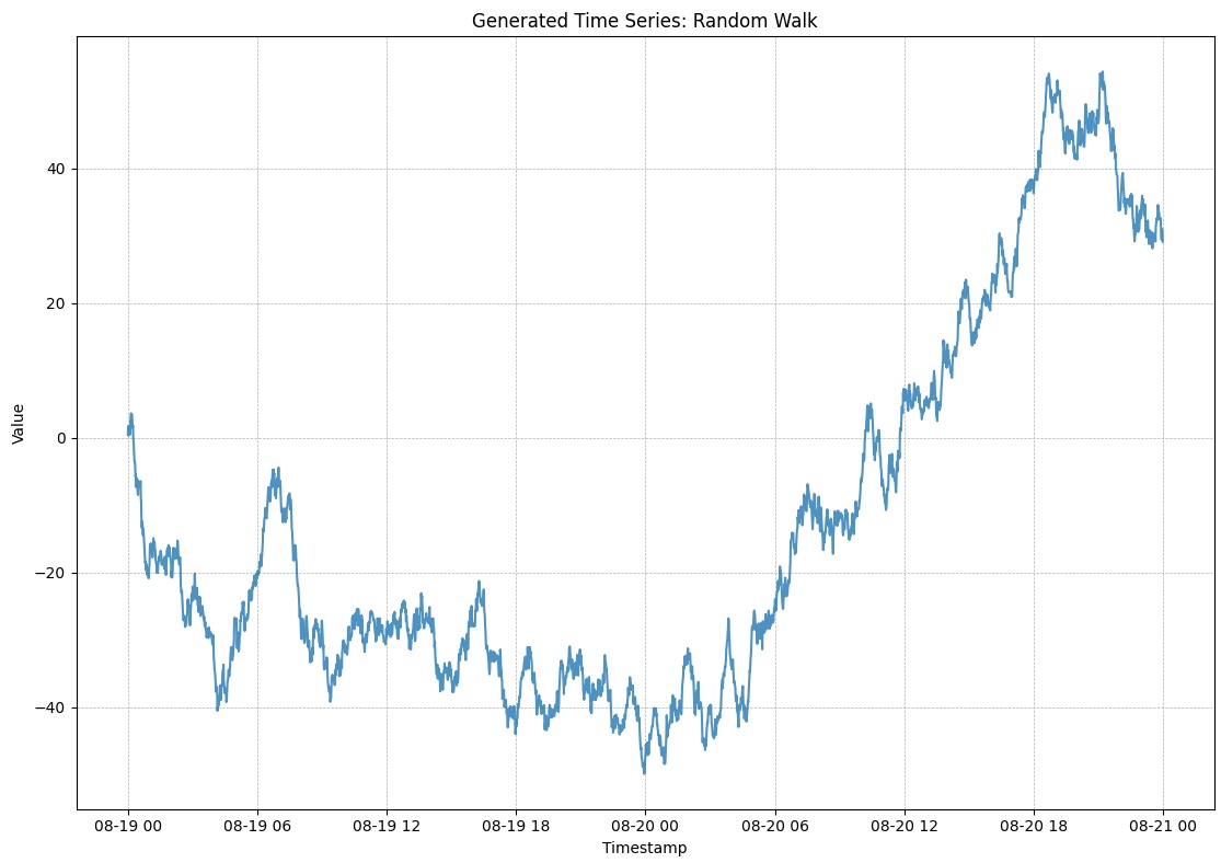
This gives some nice looking results:

Variations on the Random Walk

Laplace

In the basic version of our random walk we used the Normal or Gaussian distribution. The Gaussian distribution is the bell curve. The majority of the probablity density is centered around the mean.

There are other distributions that are symmetrical (i.e., generated both positive and negative values) and have a different behaviour than the Gaussian distribution.

For example, the Laplace distribution is very spikey around the mean and has long tails. In other words, it is more likely to generate values around the mean, which we’ll typically choose close to zero; but is has a non-negligible chance of hitting a big negative or positive value.

The expected result of a random walk with the Laplace distribution is thus a time series that varies more slowly than the random walk with the Gaussian distribution. But it will have bigger jumps (up- and downward), from time to time.

Here is a code snippet to generate a Laplace Random Walk:

import numpy as np
timestamps = utils.generate_timestamps_vectorized(
    start_date, end_date, time_step, jitter
)
n_samples = len(timestamps)

loc = 0  # mean
scale = 1  # standard deviation equivalent
values = np.cumsum(np.random.laplace(loc=loc, scale=scale, size=n_samples))

Other distributions

There are many other distributions that are symmetrical and have a different behaviour. However, even non-symmetrical distributions that only generate positive numbers, such as the Poission distribution, can be useful.

The Poisson distribution is typically used to model the occurrence of events in a given time frame. As such, it is a perfect candidate to make a time series that simulates an error counter in a software monitoring setup.

tsmaker

All the charts were generated using the time series generator tsmaker (an open source Python package & CLI tool).