Inverse Fourier for Repeating Pattern

The Fourier transform decomposes a signal into a sum of weighted sine waves. The rational behind the method is that slow moving sine waves capture the general trend of the time series. Whereas the fast moving sine waves capture the details in the time series.

Why decompse a time series into sine waves? Noise is seen in the details. Thus, removing the fastest moving sine waves corresponds to removing noise. Denoising is an example of a function that is easily implemented/expressed on sine waves, but very difficult on the original time series.

In this blog post, we will use the inverse of the Fourier transform: starting from a set of sine wave, we re-compose the time series. The contribution of each sine wave in the set is randomly chosen.

This is not a deep dive into Fourier transforms. There are better resources to be found to get a good explanation of Fourier transform. As a result, the explanation is a bit hand-wavy, but we will get to the implementation quickly and you’ll understand enough of Fourier to follow along.

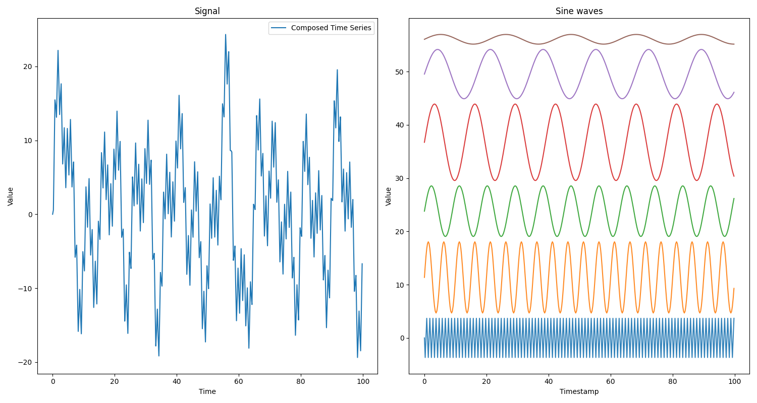On the left the time series composed by summing the sine waves on the right. Do note that the sine waves of the right are offset from the x-axis to be able to view them separately. In this case there are 6 sine waves with different periods, order from shortest period at the bottom to longest period at the top. Each sine wave is multiplied with its coefficient (coefficients = [3.6778217 6.68162936 4.75042467 7.17927268 4.62369844 0.90768227]).

Generating a time series in the Frequency Domain

A Fourier transform, maps the time series into the frequency domain. Roughly speaking, the frequency domain is the set of weights assigned to the different sine waves.

Likewise, the inverse Fourier transform, maps coefficients in the frequency domain into a time series. As a result, to generate a random time series, with a repeating pattern, we can choose a random set of coefficients in the frequency domain, and map it back to a time series.

The period of a sine wave is the time it takes for it to go up, down and back to zero. A long period means broad strokes, general trends. A short period means fast up and down moving, hence, details in the time series.

min_period_sec = ... # Shortest period of a sine wave; this is the fastest moving sine
max_period_sec = ... # Longest period of a sine wave; this is the slowest moving sine

# Different periods of the sine waves
periods = np.linspace(min_period_sec, max_period_sec, model.n_coeffs)

# Picking random amplitudes for the sine waves
coeffs = np.random.uniform(-1, 1, model.n_coeffs)

# Adding sine waves
chunk_time = np.arange(0, max_period_sec, settings.time_step)
chunk_signal = np.sum(
    coefficient * np.sin(2 * np.pi * (1 / period) * chunk_time)
    for coefficient, period in zip(coeffs, periods)
    if p > 0
)

Which generates a time series looking like this:

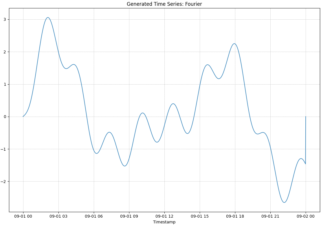
tsmaker --start-date 2025-09-01 --end-date 2025-09-02 --time-step 60 --fourier --visualize

This time series was generated with the default setting of 10 coefficients, meaning it sums up 10 different sine waves. You can still clearly see the effect of each sine wave in the signal.

Or with a bit more coefficients (100), we get a result like this:

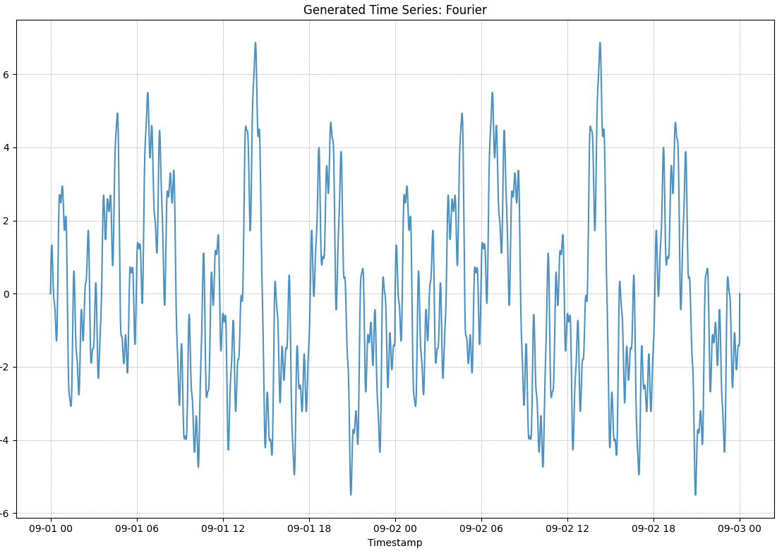
tsmaker --start-date 2025-09-01 --end-date 2025-09-03 --time-step 60 --fourier --fourier-coeffs 100 --visualize

In this case, I’ve generated two days. You can now clearly see the repeating pattern, because the maximum period of any sine wave is 1 day. This implies that the first and second day in this chart are identical, because a sine wave repeats itself after a period.

Generating complicated-looking, yet repeating patterns in a time series is the main use case of this generator.

This generator is implemented in the time series generator tsmaker (an open source Python package & CLI tool).